DARTS : Human Resources Query

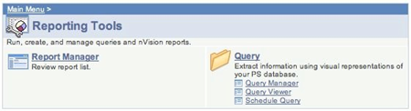
Writing a Sample HR Query

In our sample query, we’ll proceed as if we were asked to produce a list of employees for a department and needed the following information: Employee ID, Name, Job Code, Regular/Temp Status, Employee Class, FTE, and Employment Status.

Planning can be simple, you may just need to determine which fields you need and which records those fields are in.  For more complicated queries, you may need to decide which tact to take beforehand.  A query asking for all vacation time taken by employees in the engineering college might be better approached by finding all of the engineering employees and then their vacation time, a query with a wider scope might be better approached by first finding reported vacation time and then finding the employees that match that criteria.  

There are basic questions that should be answerable before writing queries:

What are ‘Active’ employees?

Employees might be on leave, on sabbatical, suspended or on work break.  Should they be counted?  

Should you count temps? Students? Graduate Assistants?

What constitutes your faculty? Coaches? PATFA? Non-represented part-time?

When you are asked for numbers do they want headcounts or FTE?

Always consider who will be reading your data.  Will they understand the codes or the terms used?

The PATFA issue:

• Some are temporary, some are regular

• Many have multiple Active Jobs; this includes different HR Departments and Campuses.
• The FTE listed on each Job Record has not been consistently or accurately maintained.

• The all have a union code

• They are in status ‘Active’ while on break.  This accomdates poulation of  PATFA Union Service Lists for a total of 6 Academic Year Semesters regardless of contined teaching.

• They are ‘faculty’, the term "adjunct" is not used in HR.

There are many more issues depending on the data you are looking at.  Each campus should decide how they want to cover these issues and adhere to standards so data retains some consistency from one query to another.

Find your Data

In this case, I’ll let you know that virtually all of our data can be found in a record appropriately named JOB.

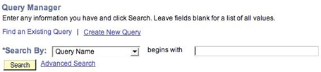
To start our query, we want to click the ‘Create New Query’ link in the Query Manager as shown in Figure 3.

 Figure 5, Selecting a Record

Upon starting a new query, the tool instantly asks you to pick a record from which to start.  For most queries, you will want to start with a record that will give you as many of the fields as you need, or holds the fields that will act as the majority of the criteria.  Fields do not need to be returned by the query in order to be used as criteria.

 Figure 6, Selecting Your Record

In this case, we do want the JOB record, so click ‘Add Record’ to use it in your query.  If you’re trying to find a specific piece of data and do not know if the record has what you need, ‘Show Fields’ will list all of the fields in the query.  Also note the ‘Advanced Search’ link, you can use that find records which contain a specific field.

 Figure 7, Effective Dating Warning

Whenever you use a record that has effective dating, you will get this warning.  What is important to know when you see this message is that the database will automatically give you the very latest dated row for the criteria.  If you remove the effective dating criteria, this query will return every job row ever created for the employees you select.  We will look at the criteria later and examine its effect and drawbacks.  For now, simply click OK.

 Figure 8, Selecting Fields from the Query Tab

For simple queries, you can actually do almost everything you need right from this screen.  Simply put a checkmark in the box next to the fields you want, and remove the check field for any fields you found you did not need in the query.  If you don’t mind a lot of data you can even click all of the fields in a record.  But be careful, there are limits on the amount of data you can return in one query. You can even remove the entire record by clicking the minus sign all the way to the right of the record name.

Pressing the icon of a minus folder will collapse the fields if you want to hide the fields.  The most useful on this screen is the little box up above the records labeled “A-Z”.  Press that and it will put the fieldnames in alphabetical order making it easier to find the specific fields you need for your query.  

For our query, you’ll need to find the following fields in the JOB record:

• EMPLID

• DEPTID

• JOBCODE

• EMPL_CLASS

• EMPL_STATUS

• FTE

• and the field that determines if an employee is regular or temporary.

What doesn’t exist in the JOB record is any personal information on the employee.  One of the goal of databases is not to be redundant; it doesn’t make any sense to store data in multiple places, even if it would be more convenient for the query writers.  So while there may be many job rows for an employees, it would waste space in the database to store the employee’s name (and other piece of personal information) every time an update was made, instead each row has an EMPLID.  The name is stored (with any changes) in a separate record.  For our purposes, we will use the record PERSON_NAME to get the employee’s name.

Navigate to the tab labeled ‘Records’ and search for this record and click on ‘Show Fields’

 Figure 9, Show Fields

Looks like it has what we need.  Click ‘Return’ and ‘Join Record’

 Figure 10, Creating a Join

When you add the record, it asks you how you want to make the join.  You can either do a standard (inner) join or an outer join.  It is also asking you which record to join to.  We want a standard join, so you simply need to click on the JOB link.

 Figure 11, Join Criteria

After selecting the records to join, it will then ask you for the fields to join.  At this point it might be useful to note the aliases, or record indicators.  If you look closely at Figure 8, you’ll notice that JOB was assigned an alias of A. Database programmers use aliases extensively because it saves typing, the query tool uses aliases because it allows for more information to be presented on the screen.  What the screen above is telling you, is that it will join two records: JOB, which it will call A, and PERSON_NAME which it prefers to call B, and will perform the join by making sure the EMPLID in both records are equal.  That is exactly what we want, so clicking the button labeled ‘Add Criteria’ will allow us to select fields from PERSON_NAME.  When you select a name (from the many choices!), use NAME_PSFORMAT for our example.

Tip: Be careful when doing joins, sometimes Query is too helpful and tries to put too many fields in the join criteria.  You always need at least one piece of join criteria, but too many (say on fields we don’t use in our implementation of PeopleSoft) will quickly reduce you zero data being returned. 

Tip: PS Query will  ALWAYS auto-join Effective Date Criteria as an Inner or Standard Join. The user will need to change this crtieria to an Outer Join manually when needed.

Add Your Criteria

 Figure 12, The Fields Tab

We will go to the fields tab to add the first criterion to our query.  The little funnels allow us to add a criterion to a specific field.  Note that we can only pick the fields we previously selected here.  If we wanted to add criteria based on fields that we do not want displayed, we should return to the query tab and use the funnels there.

Figure 13, Criteria Choices

The criteria screen presents us with many choices.  Basically we need to form an equation in the form of X (CONDITION) Y.  If X and Y meet the condition then we want the data, otherwise, that data will not be returned by our query.

X is called ‘Expression 1’ in Query’s terms, and by using the funnel it has already pre-filled that side of the equation with the DEPTID field from record alias A (JOB). 

Equal to/Not equal to

The most basic condition and does a check for equality.  For numbers it is compares to any available decimals, e.g. 10.00000001 is not equal to 10, and any text must match in length and case.

Between/Not between

Perfect for date ranges, and in some cases when looking at financial transactions to find a range of activity between two levels.  Note that between includes the values you use.  Using between and looking for job rows dated between 1/1/2006 and 12/31/2006 will find entries on those dates as well as those between them.

Greater than/Less than

Great for finding large payments, or transactions less than zero.  Asking for dates greater than 1/1/2006 will not find anything on that day, only starting 1/2/2006 and later.

Not greater than/Not less than

“Not greater than” means “less than or equal to” and “not less than” means “greater then or equal to.” Got that?

Is null/Is not null

Dates can be null -- this lets you find them or ignore them.  See the Zero/Null/Blank discussion in Section VI.

In list/Not in list

Allows you to pick among a list of options, we’ll explain more fully below.

Like/Not Like

Like allows us to match strings based on partial matching.  For example, using Like and ‘O%’ for our constant criteria will match every value that begins with an O – that would be perfect to find every department on the Orono campus.  

Exists/Does not exist

This bit of criteria can only be used with subqueries, basically it asks if X exists (or doesn’t) in another query.

In tree/Not in tree

I know of no reason to use this with Human Resources data, but its intent is obvious.

After setting our condition, which will be ‘Equals To’ for our example, we can set ‘Expression 2.’  Make sure that your expression type is set to ‘Constant’ and enter your department code in the box.

Save the Query

This step is completely optional just as choosing to listen to your instructor the first time you go skydiving is optional.  All I’m saying is that I don’t recommend skipping it.

Use the ‘Save’ button at the bottom of the page to save your query.

 Figure 14, Saving Your Query

The minimum you are required to do is provide a name for the query.  If you are saving a ‘private’ query that only you can see, you can pick any name you want.  Public queries should begin with ‘UM’ and you should do your best to create a description that succinctly describes the query.  For now, just keep it private and use whatever name you like.

Now you can run your query by clicking the run tab on the right side of the query menu.

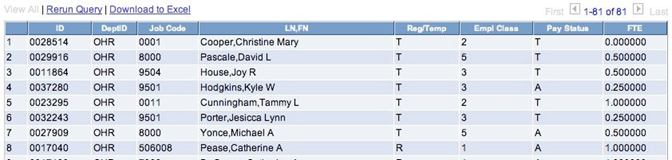
 Figure 15, Sample Query Data

If you return to the fields tab (Figure 12), you’ll notice that there is a column labeled XLAT, this indicates whether or not the database will translate the value of the field into a human readable form.  An N indicates that translate is available but not being used.  Use the edit button to translate the field.  Let’s translate EMPL_STATUS to make our query more readable.

 Figure 16, Translate Options

All you need to do is choose if you want the ‘short’ or ‘long’ translation of a name.  In almost all cases the short name will be enough.  When you return to the Fields tab, you’ll notice that the XLAT column now indicates S for a short translation.

Only fields which have a value in the XLAT column can be translated.  However, query also can suggest tables for possible translation as well.  If you return to the Query tab and look at the fields in the JOB record, you’ll notice that certain fields have a recommended job option to the right of the field name.

Figure 17, A Suggested Join

In this case, let’s join JOBCODE to its own data table.  We can add the DESCR field and use it to provide more information in our query.

While our original specification did not specify one way or the other, it is probably safe to assume that we only want active employees.  This gives us a chance to use another criteria type.   Add criteria for the EMPL_STATUS field and pick the condition of ‘in list’.  You can’t type your Expression 2 here, you have to add your items from a list.  Click the magnifying glass to get your choices.

 Figure 18, List Selection

When you select your choices, normally Query will give you a list of possible values.  In this case it also provides the long and short translations of the fields values.  Click ‘Add Value’ for any values you want to include in your query.  For ‘active’ employees, I try to remember the mnemonic ALPS+W, other combinations may be more appropriate for your campus or your specific needs.  

 Figure 19, Sample List Criteria

When you’re done selecting values, the criteria should look like Figure 19.

 Figure 20, Reorder Fields

One thing you can do to improve the readability of your query is to reorder the fields.  I like to have key fields, such as EMPLID and NAME to the left.  It also makes more sense to have the JOBCODE close to its own translation field.  To change the order of the fields, navigate to the Fields tab and click the button labeled ‘Column Order.’  Figure 20 shows the order of fields as I originally selected them and my preferred column order in the boxes on the right.  

 Figure 21, Sort Order

The Fields tab also has an option for sort order.  You can get your data pre-sorted from the query and not need to sort it later when you bring the data to Excel or other software on your computer.  In Figure 21, you can see the NAME_PSFORMAT field has been designated as the primary sort and that it will sort Ascending (starting with A.)  The reason we selected the NAME_PSFORMAT is that the fact it places the last name first it lends itself to sorting.

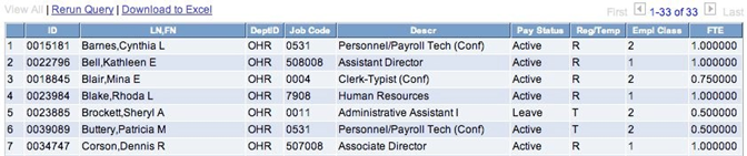
 Figure 22, Modified Query

After making the changes, you can see that the fields have been reordered, we are getting many less employees and the names are now sorted.

 Figure 23, Adding a Prompt

An important consideration when writing queries is that a query should be reusable.  One of the easiest way to enhance a query is to add a prompt value which will allow you to change one or more pieces of criteria without having to re-edit the query.  This also allows individuals who can not edit queries to use your query for multiple situations.  Since our query reports on the employees in a department, we’ll change the query so it asks which department we would like to report on.

Navigate to the Criteria tab and click the ‘Edit’ button next to the DEPTID field.  Then change the Expression 2 type from Constant to Prompt.  In this case we want a New Prompt, so we will click that link.

 Figure 24, Defining a Prompt

We can leave the criteria as it is.  You might want to change the ‘Heading Text’ so it gives a more readable prompt to the user.

Save your query and try running it.

Unfortunately, this points out one problem with the prompt system.  It tries to guess at what you are doing and occasionally gets it wrong.  What it is trying to do is make sure that the department code you entered is valid by checking it against the departments listed in DEPT_TBL (see Figure 24).  Unfortunately, in our system we don’t have access to DEPT_TBL. You have two options to resolve the problem, you can change the ‘Edit Type’ to ‘No Table Edit’ or you can change the ‘Prompt Table’ to ‘SET_DEPT_VW’.  Either will work.  The advantage of the latter option is that it retains the ability to search for valid values.

Most prompts you setup won’t need this extra detail, you will be able to setup a prompt and go.  Prompts are especially powerful when used with date ranges.  Also note that the ‘Format’ value in the prompt criteria – that tells Query to override what the user enters and make it all capitals.  This prevents you from having to explain to each user the importance of using the proper case with query.

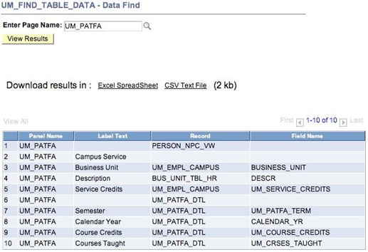
Arguably the most difficult part of writing query is just trying to find the data you want to query on.  There are several options.

Click on Look up the Data for information on Finding Your Data.

Flat File

There is a special record named UM_F_EMPL_VW that was especially created by the tech team to make querying easier.  It combines many of the most commonly used fields into one table, and in many cases even includes the translation fields separately.  The term ‘flat file’ originates because the data has been flattened, meaning there is no history – you always get the latest data. 

There are disadvantages to using the flat file.  The most obvious issue is that it offers no way to look at history.  Also it isn’t as friendly as other records – you may not get a list of options when creating an option and there are little to no suggestion joins for bringing in other data as we did above with JOBDATA.

In many ways however, using the flat file is the future of Query, both in its ease of use and speed as well as the flat file being the foundation of the Discoverer tool.

HR-Query Mailing List

Ask Kevin Foss (kfoss@maine.edu) and he’ll add you to the mailing list set up for individuals who write queries against HR data.  You can ask questions about finding data, methods of using query or simply ask if others have tackled a specific problem before.

Letting the Database Help You

Aggregates

Query can do some calculations for you.  When you are looking at the fields tab, one of the options is to click the ‘Edit’ button (this is also how you get to the translate options) and create an aggregate calculation on a field.

Figure 28, Aggregate Choices

This allows you to apply one of the aggregates to a column in the table.  Note however, that it aggregates values only if every other field is the same.  Consider our earlier example – we are returning a unique EmplId and Name for each row.  Adding an aggregate to FTE, to summarize the total FTE count in the department would do nothing to our query as is – it would only sum the FTE for each individual and produce the exact same results.

However, if we were to remove every field except department and FTE and turn on the ‘Sum’ aggregate, our output would look like this:

 Figure 29, Sample Aggregation

Now, imagine if we were to remove the criteria to prompt on department.  Then our query would summarize the FTE for every DEPTID available (depending on security.)  However, you should really consider if this query would really be the best for the job or it would be better to start over and write a new query.

The other aggregates are also useful:

Count

Will count the number of values that match each row returned.  Changing our query to ‘Count’ instead of ‘Sum’ FTEs will effectively return a headcount for a department.

Average

Will produce an average (arithmetic mean) of the values.

Min/Max

Can be used to find the minimum and maximum values – you might use this to find the lowest and highest paid individuals in a job code or salary grade.

Aggregates are useful, but in some ways that are very limiting.  All of these functions and many more are available in any spreadsheet software, and it may be useful to bring raw data back and summarize and analyze data there rather than directly in query.

Note that aggregates should only be used on fields which make sense to be aggregated, there is no concept of a ‘Min’ name field or an ‘Average’ date in a database.

Column Headings

When editing columns, there is a third option that allows you to change the heading of a column.  Again, you want to click on ‘Edit’ next to a field and in this case we will be changing the heading for NAME_PSFORMAT as by default it prints the unintuitive ‘LN,FN’ designation (Figure 22).

Figure 30, Heading Option

In this case, we have selected the heading should be ‘Text,’ which means it will use the value we type in the ‘Heading Text’ field.  This change will affect how the column headings appear both on screen and in any file export.

The usefulness of this feature again is limited, as these changes could as easily be done on a spreadsheet, but if you are running a query routinely and editing your spreadsheet headings every time, then making this one change would save you from that task in the future.

Expressions

There are two major uses for expressions:

• Do simple calculations on fields

• Use database features not directly accessible from the Query interface

The second option will not be covered in the course but is one of the most powerful features of query.  

The first option allows you to do simple manipulations of the data to produce new values.  Consider a request to determine what the impact of a 2% raise on all of the salaries in a department would be.  You would first find the field that gives an employees salary, and then could create a mathematical expression.  Navigate to the ‘Expressions’ tab and click ‘Add Expression’.

 Figure 31, Adding an Expression

Be mindful of the expression type and length.  The type needs to match your data.  As with aggregation, expressions should only be used when they make sense.  It simply will not know what to do if you try to multiple a name field by 80 hours but it will allow you to create such an expression.  The error won’t be flagged until you run the query and get a (sometimes unhelpful) error message. As much as any other area in query, you need to plan what you are trying to achieve before using an expression.

The ‘Length’ value determines the length of the field, and the ‘Decimals’ is used for numeric fields when you want a certain number of decimal places in your result.   The decimals subtract from the overall length.  A number defined as 4.2 will hold numbers from 99.99 to -99.99.  You can find how values are stored in the database by looking at the ‘Fields’ tab. (Figure 12)  Although be warned they are using a different notation, a 4.2 on the ‘Fields’ tab means 4 places to the left of the decimal and 2 to the right, or a 6.2 expression.  Lastly, just because a field always uses number, it may in fact be stored as a character string.  

For our example, click the ‘Add Field’ link and find ANNUAL_RT in the job record.  Using 8 and 2 for the length and decimals of a number field will be sufficient.  Your expression should like this:

 Figure 32, A New Expression

Note that we did the math in the expression just as we would for a formula in Excel.  For general usage, simple arithmetic will be the same.

Expressions do not even need to involve fields that already being returned, but do need to use fields in the records you have selected.  Unfortunately there is no way to determine the native type of a field without making it a returned field so you can review it on the ‘Fields’ tab.

Essentially by creating an expression, you have created your very own field.  As you can see from looking at the updated ‘Expressions’ tab, the value can be returned (click on ‘Use as Field’) or you can apply criteria to the value.  By creating this expression, it will perform this equation on the annual rate for every row, and any criteria will be applied accordingly.

 Figure 33, The New Expression Ready To Use

Again calculated expressions may be better served in a spreadsheet after compiling the raw data, but by using criteria on the expression we can greatly reduce the result set.

Data is not created equal, and that is never more apparent then when you are looking at (or for) nothing.  In database terms, an empty field, a field with the value of zero or a field whose value does not exist (null) are all different things.  To a human that all express absence of data, but to a database they all carry their own nuances.

Text (character) fields can either be set with a value or they can be empty.  To find text fields with no values, say missing title fields, you will need criteria looking for an empty string.  An empty string is represented by ‘’ when you review the criteria. To enter an empty string simply use the ‘Expression 2’ section blank and use what ever condition is appropriate.

Number fields always have a value, and should be stored as zero if no value is available.  As mentioned in the discussion in Expressions, some fields that happen to only use number may actually be strings so to test those fields you’ll need to look for empty strings.

Dates either exist or do not exist, unlike numbers there is no default date and no way to logically convey a date that is empty.  So you need to use the conditions that check for null values in order to find blank date fields.

Effective Dating

Successful query writing depends on knowing how the data is organized and stored in the database.  Effective dating may be the most important concept because it is the overriding factor in what you get for data.  For most queries, you will want the most current data so letting Query set the effective dates in use (or using the flat file) is completely appropriate.  However, at times, effective dating can get in the way of allowing you to get to the data you need.

When you add a record with an effective date, the following criteria is added:

 Figure 34, Effective Dating

Effective dating has its own class of condition type, and in this case it is asking for the row with the last effective date less than or equal to the current date (i.e. today) and the last sequence number for that date.  It excludes future dated rows.  It is entirely possible to ask for rows that were between a date range, on an exact date, or remove the effect dating criteria entirely.Y ou might want to look at a range of dates to find all of the new student hires done in a month – looking at the current row may only give you rows with minor data corrections but not the actual hire row.  You might want to review across-the-board actions and only look at rows for a certain date, but almost instantly the latest rows will be something else as the result of ongoing data maintenance.  Luckily it is as easy to change effective dating criteria as any other criteria, but you need to know the ramifications.  Removing the criteria completely would have found every row generated for every employee in our department listing example.  Even looking at a range of dates, it is difficult to pick out the latest row (aggregates won’t work) so the best you may do is to get one row for most individuals and 2 or more rows for some of your rows. You also have to consider effective dating when joining tables.  Overtime, values change in the database and the latest job row for an individual may be from last year, but the table holding job descriptions may have been updated yesterday.  The effect may be minor, but you may end up with data that looks ‘different’ in your query results then how the same row appears on the user screens if you depend on effective dated translation. The other major consideration with effective dating is that for technical reasons, a record which has effective dated criteria can not be used in an outer join.  This stipulation does not apply to the flat file.

Excel/CSV

There a several options for return data from a query.  You can have it placed directly in to a spreadsheet by clicking on the ‘Download to Excel’ link, visible in Figure 29.  Any values are brought over as-is, so if you did any calculations or sorting you get the values after the changes have been applied.  The Excel option is available any where you run a query.In some cases, it might be worthwhile to get data that is better suited for easy manipulation in an external database.  The data can also be accessed in CSV (Comma Separated Values) format.  The easiest way to get a CSV file is to run the query from either the Query Viewer (link shown in Figure 2) or by using the ‘HTML’ option in the Query Manager (obscured in Figure 37) when finding a query, i.e. before you edit it.  CSV files are smaller and more universally compatible then Excel files.Managing Your QueriesCopyingNever change (and never, ever break) someone else’s query.  There are many great public queries available in Query Manager which have already been written.  Using what you know about how to find data, and searching for queries, it should be easy find other queries using the same concepts you want to use.  However, if you can only find queries kind of like what you want you should resave (and rename) the query in your own library.Use the Save As link at the bottom of query to resave a copy.

 Figure 35, The Save As Screen

In this case, to save a copy you would want to change the name and change the owner to ‘Private’.  I often change queries by adding my initials so I know it is my own variant. After you’ve saved you can begin to make modifications.  

Don’t worry, I will know if you resaved my query.  While I put in my email and initial creation date, you can easily find the creator (and last save date of any query.)  When you are editing the query, there is also a link called ‘Properties’ – click that and you’ll see all of the information above as well as the following information:

 Figure 36, Last Update Information

That tells me that the query was last saved in March of last year, and I made the change.  All queries have this information and can be a valuable tool if you need to ask a query writer a question.  I use the update date in case I find I have a bunch of queries with similar names but don’t remember which one I used most recently.

Private queries can not have the name of any public query, keep that in mind when naming in your queries.

Now using save as is a great way to get queries into your own library, but what if you want to copy a private query to someone else who can’t edit their own queries?  You can either make the query public (and don’t do that if you haven’t made the query generally applicable) or you can copy the query to their library.

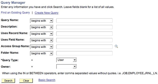
First you need to find the query in the Query Manager:

 Figure 37, Query Manager

Note the action drop down box you have several choices here.  If you select ‘Copy to User’, select the checkbox next to the queries you want to copy and click ‘Go’ you will be prompted with the following screen.

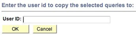
 Figure 38, Copying a Query

Renaming

Renaming queries is very easy.  Simply select the query you want to rename and choose the ‘Rename Selected’ option.  The screen looks like this:

 Figure 39, Renaming a Query

Folders

Queries can be saved in folders for easy organization.  After selecting the ‘Move to Folder’ option you will be presented with the option of using a new folder, or creating a new folder. 

Figure 40, Moving to a Folder

If I am now searching for queries, I have more than 300 and can only view the first 300 queries in the system.

 Figure 41, Without Folders There Are Too Many Queries

Changing my Folder View to just look at the ‘Test’ folder I created in Figure 40 I can easily find my queries.

 Figure 42, Queries in a Folder

Imagine if everyone filed their queries into folders appropriate if they were a ‘Benefits’ or ‘Payroll’ query, or if campuses kept their own folders?

Add to Favorites

When you move queries to a list of favorites, you will be greeted with this list of queries as soon as you enter the query manager.

 Figure 43, My Favorite Queries  

Deleting Queries

Don’t.

Unless they are your own, then okay, delete away.  We do have too many public queries so clearing out the deadwood is always a good idea.  

Your First IPO

Public queries are a good thing but they should also only be saved publicly if they are useful for other people.  Public queries should not be tied to one campus either in the specifics of its criteria or in the data it uses.  Good public queries should have general applicability by using prompts to specify business units, departments and date ranges.  Assumptions shouldn’t be made about what the user wants to report on.

Public query should cover situations that will come up again and again and not just to answer one specific question.

With previous versions of query it was not possible to copy queries to individuals who can not edit queries so many queries were made public for that reason alone. 

By minimizing the use of public queries, it should be easier to find the quality queries that we can all use and learn from.  It will also lead to less duplication if it easier to tell if others have written the queries to tackle the same problems.